TROSY EXPERIMENT
Here are step-by-step instructions how to reproduce the
ab_hsqc_abtp
TROSY-type experiment, suggested in
Anderson, P., Annila, A., and Otting, G. "An a/b-
HSQC-a/b experiment for spin-state selective
editing of IS cross peaks",
J. Mag. Res. 133,
364 (1998).
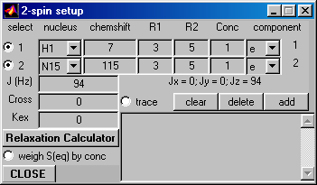
Select your spin system using Spin System Setup Window. The example shown here simulates
a TROSY spectrum for a pair of 1H and 15N nuclei, with 94 Hz scalar coupling. If you want
to merely simulate selection of particular transitions in a TROSY-type experiment, you
can use the default values of spin-relaxation parameters.
Relaxation Calculator:
If you also want to take into account the differential line broadening effects for different
spin-doublet components, click on the Relaxation Calculator button, select desired dynamic
parameters, and Calculate relaxation rates. Then check out the R2-matrix button (as shown
below) and click on the Update button. For more details of how to use Relaxation Calculator
see the example of a Fully coupled HSQC experiment with spin-transition-specific linewidths.
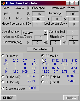
Note: This T2-relaxation matrix does not properly reproduce relaxation rates for the
double-quantum (I+S+, I-S-) and zero-quantum
components: this bug will be fixed in the next VNMR release. This, however, is not
important for the demonstration of the Trosy-type signal selection.
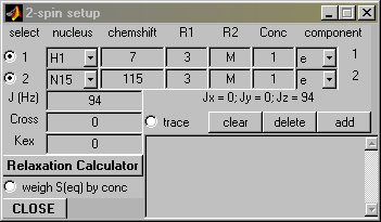
Check the Spin Setup Window:
The boxes for the individual R2 values should contain letter "M" (i.e. matrix) instead of numeric values.
Pulse Program: Experiment A
Now let's go to the pulse program.
Select the ab_hsqc_abtp pulse program. Edit the phase cycling lines of the program so that phase cycle "A" is selected (i.e. you have to uncomment the pair of phase cycle lines labeled "A". Make sure that all phase-cycle lines labeled "B","C", and "D" are commented out!).
The relevant lines should read:
ph14=1		;A

ph15=0		;A

;ph14=3		;B

;ph15=2		;B

;ph14=3		;C

;ph15=0		;C

;ph14=1		;D

;ph15=2		;D
Now click on Xlate button to translate the pulse program into Matlab code.
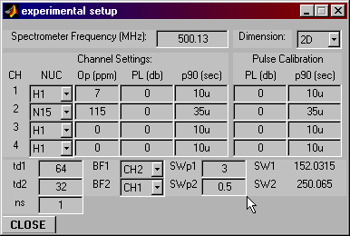
Set the Program Parameters as follows (change nd0 to 2, set d1 to 3s and d4 to 1/94/4,
which equals 1/(4J)) :
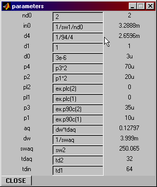
Experimental Parameters:
Op1=7, Op2=115, td1=64, td2=32, ns=1, BF1=CH2, SWp1=3ppm SWp2=0.5ppm
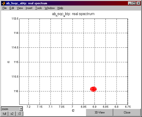
Run the experiment. Now store the "A" spectrum by typing the following at the command line:
serA=vs_runCalc.ser0;
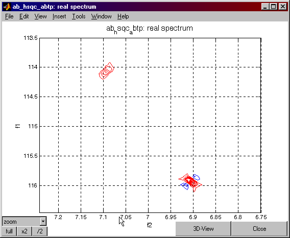
The spectrum from the A data set should look like the following (process using TPPI):
Pulse Program: Experiment B
Now edit the ab_hsqc_abtp pulse program again to select the "B" phase cycle.
Once again the relevant code should be:
;ph14=1		;A

;ph15=0		;A

ph14=3		;B

ph15=2		;B

;ph14=3		;C

;ph15=0		;C

;ph14=1		;D

;ph15=2		;D
Translate the pulse program again (you have to translate it every time you change the pulse program!), reset the program parameters as before, and then run the experiment. You do not have to reset the spin system parameters or the experimental parameters -- they have to (and will) remain the same as in experiment A.
Once again save the B data set by typing at the command line:
serB=vs_runCalc.ser0;
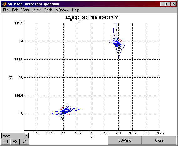
The raw spectrum from the B data set should look like the following (process using TPPI):

Repeat the above process to create and save a "C" data set:
(1) edit the pulse program in order to select the proper phases (marked with ";C");
(2) translate;
(3) set the program parameters;
(4) run the experiment;
(5) type serC=vs_runCalc.ser0;.
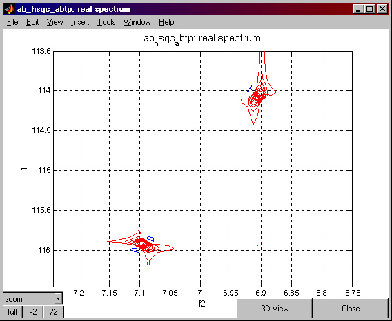
The spectrum should be similar to the following:
Finally, repeat the process for the "D" data set:
(1) edit the pulse program in order to select the proper phases (marked with ";D");
(2) translate;
(3) set the program parameters;
(4) run the experiment;
(5) type serD=vs_runCalc.ser0;.
Combining the data sets: Let's do the magic
Now that you have the four data sets (serA, serB, serC, serD), you can combine them to produce
the four possible TROSY spectra. The following are step-by-step instructions. (You can copy
and paste the lines to be entered at the Matlab command line.)
First, to display the anti-diagonal peaks one would:
At the Matlab command line type:
aa=serA+serB; bb=serA-serB; aa90=-i*aa; vs_runCalc.ser0=aa90;
Press the PROCESS button on the Data Processing Window.
At the Matlab command line type:
PPa90=vs_runCalc.spe; vs_runCalc.ser0=bb;
Press the PROCESS button on the Data Processing Window.
At the Matlab command line type:
PPb=vs_runCalc.spe;
At the Matlab command line type:
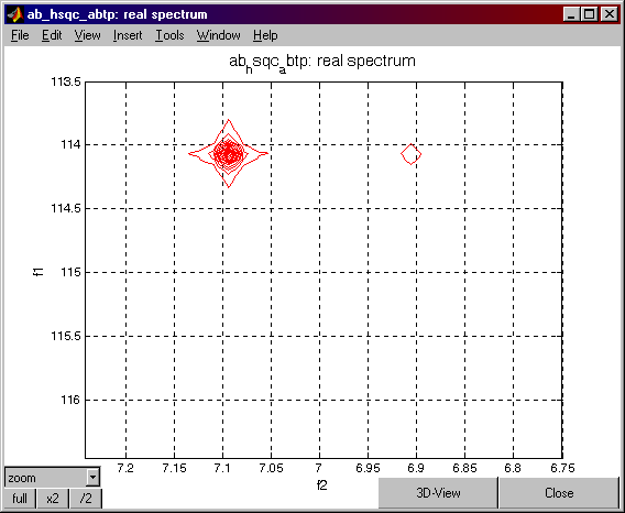
vs_runCalc.spe=i*(imag(PPb)+real(PPa90))+real(PPb)+imag(PPa90);
Press the REAL button on the Data Processing Window. The following spectrum should appear:
At the Matlab command line type:
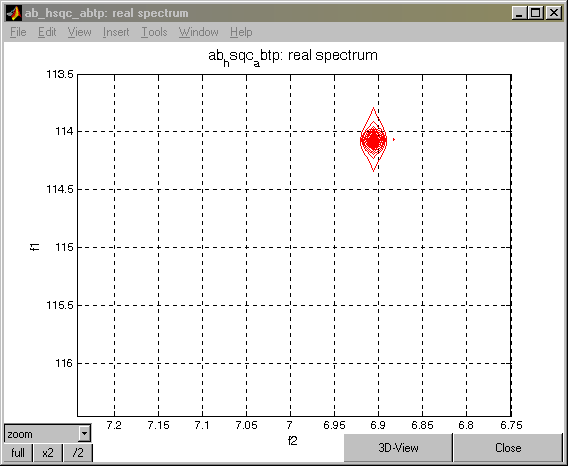
vs_runCalc.spe=i*(imag(PPb)-real(PPa90))+real(PPb)-imag(PPa90);
Press the REAL button on the Data Processing Window. The following spectrum should appear:
To display the other two multiplet components one would:
At the Matlab command line type:
cc=serC+serD; dd=serC-serD; cc90=-i*cc; vs_runCalc.ser0=cc90;
Press the PROCESS button on the Data Processing Window.
At the command line type:
PPc90=vs_runCalc.spe; vs_runCalc.ser0=dd;
Press the PROCESS button on the Data Processing Window.
At the Matlab command line type:
PPd=vs_runCalc.spe;
At the Matlab command line type:
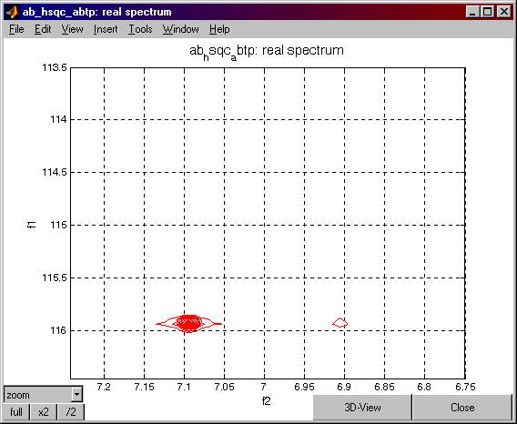
vs_runCalc.spe=-(i*(imag(PPd)+real(PPc90))+real(PPd)+imag(PPc90));
Press the REAL button on the Data Processing Window. The following spectrum should appear:
At the Matlab command line type:
vs_runCalc.spe=-(i*(imag(PPd)-real(PPc90))+real(PPd)-imag(PPc90));
Press the REAL button on the Data Processing Window. The following spectrum should appear:
Go Back to VNMR Tutorial Index
Back to Top
These instructions were designed by Peter Nicholas. Modified by David Fushman & Olivier Walker.
Last update 11/17/2002.
(c) Copyright 2002 by David Fushman, University of Maryland.