Simulating a fully coupled 1H-15N HSQC experiment with spin-transition-specific linewidths
Pulse Program: invitpHNcpl
The pulse program for this example was obtained by modifying the standard Bruker INVITP pulse sequence. Two modifications were made here:
(1) We commented out the 180-deg refocusing 1H-pulse during 15N evolution (line (p2 ph2)) . The corresponding lines in the pulse sequence look like:
(p1 ph3) (p3 ph6):f2
d0
;(p2 ph2)
d0
(p1 ph4) (p3 ph7):f2
(2) We commented out the explicit command to implement 15N decouplling during the acquisition:
go=2 ph31 ;cpd2:f2
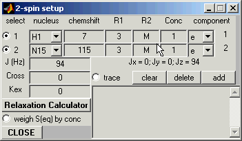
First Select the Spin System:
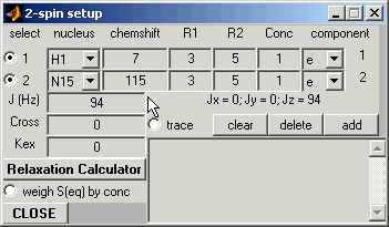
The spin system selected for this example consists of one proton-nitrogen pair. The one-bond coupling was set to J = 94 Hz.
Note: When selecting spins to input the J coupling, be sure to check them out from top to bottom, i.e. in the order of their nucleus numbers. For example, in the case shown here, select the 1H spin first and only then 15N.
Then Calculate Spin Transition Rates Using Relaxation Calculator:
In order to take into account the differential line broadening effects for different
spin-doublet components.
Click on the Relaxation Calculator button -- the Calculator panel pop up.
Important: Make sure that the spins appear in the same order as they are in the Spin Setup panel. If the order is different (e.g. in this case 15N will aper on the first line and 1H on the second), close the Relaxation Calculator, unselect both nuclei in the SpinSetup window, and then select them again, now in the right order, as described above. Then reopen Relaxation Calculator. If you don't do this, it will result in the wrong order of the corresponding elements in the final relaxation matrix.
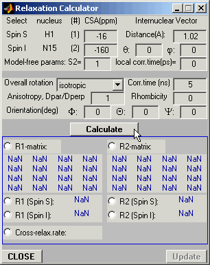
In the Relaxation Calculator panel, select desired dynamic parameters, and click the Calculate button to calculate spin relaxation rates.
The calculations take a a fraction of a second. When they are done, the corresponding fields in the lower part of the panel will be updated, and the Update button will become active.
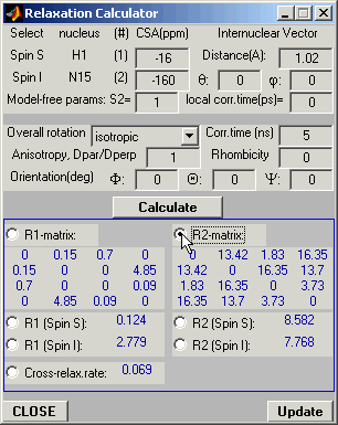
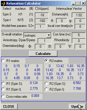
Then check out the R2-matrix button (as shown below) and click on the Update button.
Notice that for each calculation you can update the results only once. If you want to repeat the update procedure, click the Calculate button again -- this will re-activate the Update button.
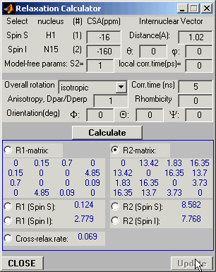
Note: This T2-relaxation matrix does not properly reproduce relaxation rates for the
double-quantum (I+S+, I-S-) and zero-quantum
components: this bug will be fixed in the next VNMR release. This, however, is not
important for this example.
Check out the Spin Setup Window
When the R2 matrix instead of the individual R2 values is put in the system (using Relaxation Calculator), the corresponding fields in the Spin Setup Window show letter "M" instead of the individual R2 values, as shown here:
Now we can start the simulation.
Select the proper pulse program (invitpHNcpl) from the vs_pp directory.
Click on the Xlate button to translate it into Matlab code.
Then open the Program Params panel and input necessary values of the pulse program parameters.
Program Parameters:
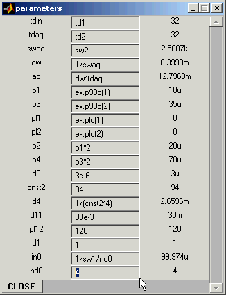
Set the following values: nd0=4, cnst2=94, d1=1s. After setting cnst2, the value of delay d4 should automatically change to 1/(cnst2*4) which corresponds to 1/(4J).
Experimental Parameters:
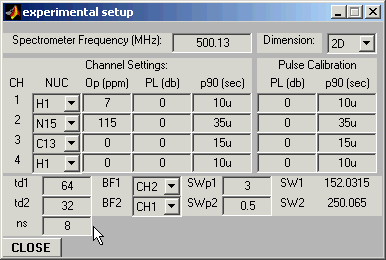
td1=64, td2=32, ns=8 (full phase cycle!), SWp1=3 ppm, SWp2=0.5 ppm, Op(1H)=7 ppm, Op(15N)=115 ppm.
Set channel 2 to 15N. Associate td1 with 15N by setting BF1 to CH2.
Data Processing:
Select TPPI for proper processing in the f1 dimension.
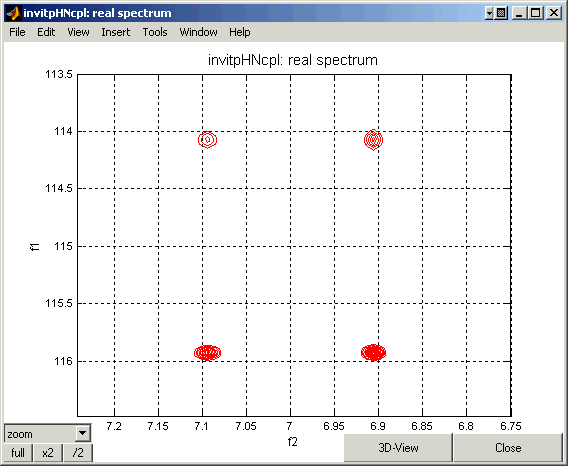
The resulting HSQC spectrum should look like this one:
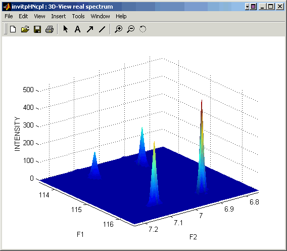
Here is a 3D-view of the resulting HSQC spectrum:
Go Back
Back to Top
Go Back to VNMR Tutorial Index
This manual page was designed by David Fushman & Olivier Walker.
(c) Copyright 2003 by David Fushman, University of Maryland.